Network devices don’t really care about the type of traffic they have to forward. Your switch receives an Ethernet frame, looks for the destination MAC address and forwards the frame towards the destination. The same thing applies to your router, it receives an IP packet, looks for the destination in the routing table and it forwards the packet towards the destination.
Does the frame or packet contain data from a user downloading the latest songs from Spotify or is it important speech traffic from a VoIP phone? The switch or router doesn’t really care.
This forwarding logic is called best effort or FIFO (First In First Out). Sometimes, this can be an issue. Here is a quick example:
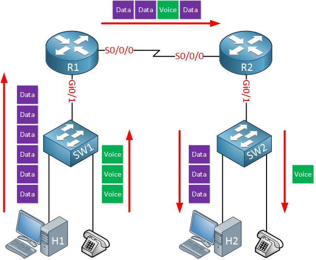
Above we see a small network with two routers, two switches, two host devices and two IP phones. We use Gigabit Ethernet everywhere except between the two routers; this is a slow serial link of, let’s say 1.54 Mbps.
When the host and IP phone transmit data and voice packets destined for the host and IP phone on the other side, it is likely that we get congestion on the serial link. The router will queue packets that are waiting to be transmitted but the queue is not unlimited. What should the router do when the queue is full? drop the data packets? the voice packets? When you drop voice packets, the user on the other side will complain about poor voice quality. When you drop data packets, a user might complain that transfer speeds are poor.
QoS is about using tools to change how the router or switch deals with different packets. For example, we can configure the router so that voice traffic is prioritized before data traffic.
In this lesson, I’ll give you an overview of what QoS is about, the problems we are trying to solve and the tools we can use.
Characteristics of network traffic
There are four characteristics of network traffic that we must deal with:
- Bandwidth
- Delay
- Jitter
- Loss
Bandwidth is the speed of the link, in bits per second (bps). With QoS, we can tell the router how to use this bandwidth. With FIFO, packets are served on a first come first served basis. One of the things we can do with QoS is create different queues and put certain traffic types in different queues. We can then configure the router so that queue one gets 50% of the bandwidth, queue two gets 20% of the bandwidth and queue three gets the remaining 30% of the bandwidth.
Delay is the time it takes for a packet to get from the source to a destination, this is called the one-way delay. The time it takes to get from a source to the destination and back is called the round-trip delay. There are different types of delay; without going into too much detail, let me give you a quick overview:
- Processing delay: this is the time it takes for a device to perform all tasks required to forward the packet. For example, a router must do a lookup in the routing table, check its ARP table, outgoing access-lists and more. Depending on the router model, CPU, and switching method this affects the processing delay.
- Queuing delay: the amount of time a packet is waiting in a queue. When an interface is congested, the packet will have to wait in the queue before it is transmitted.
- Serialization delay: the time it takes to send all bits of a frame to the physical interface for transmission.
- Propagation delay: the time it takes for bits to cross a physical medium. For example, the time it takes for bits to travel through a 10 mile fiber optic link is much lower than the time it takes for bits to travel using satellite links.
Some of these delays, like the propagation delay, is something we can’t change. What we can do with QoS however, is influence the queuing delay. For example, you could create a priority queue that is always served before other queues. You could add voice packets to the priority queue so they don’t have to wait long in the queue, reducing the queuing delay.
Jitter is the variation of one-way delay in a stream of packets. For example, let’s say an IP phone sends a steady stream of voice packets. Because of congestion in the network, some packets are delayed. The delay between packet 1 and 2 is 20 ms, the delay between packet 2 and 3 is 40 ms, the delay between packet 3 and 4 is 5 ms, etc. The receiver of these voice packets must deal with jitter, making sure the packets have a steady delay or you will experience poor voice quality.
Loss is the amount of lost data, usually shown as a percentage of lost packets sent. If you send 100 packets and only 95 make it to the destination, you have 5% packet loss. Packet loss is always possible. For example, when there is congestion, packets will be queued but once the queue is full…packets will be dropped. With QoS, we can at least decide which packets get dropped when this happens.
Traffic Types
With QoS, we can change our network so that certain traffic is preferred over other traffic when it comes to bandwidth, delay, jitter and loss. What you need to configure however really depends on the applications that you use. Let’s take a closer look at different applications and traffic types.
Batch Application
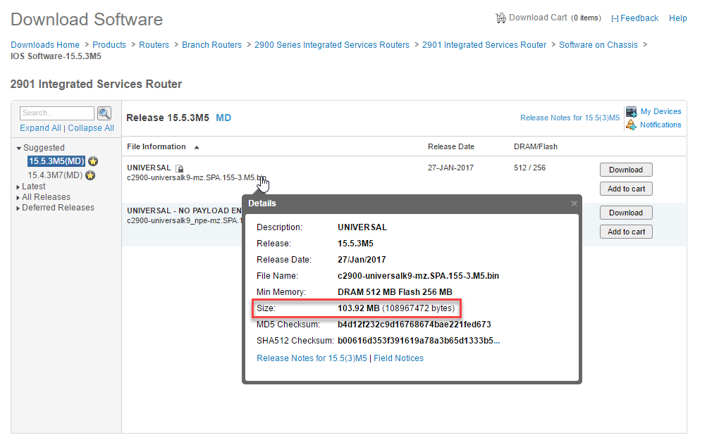
Let’s start with a simple example, a user that wants to download a file from the Internet. Perhaps the latest IOS image:
Let’s think about how important bandwidth, delay, jitter, and loss are when it comes to downloading a file like this.
The file is 103.92 MB or 108967472 bytes. An IP packet is 1500 bytes by default, without the IP and TCP header there are 1460 bytes left for the TCP segment. It would take 108967472 / 1460 = ~74635 IP packets to transfer this file to your computer.
Bandwidth is nice to have, it makes the difference between having to wait a few seconds, minutes or a few days to download a file like this.
What about delay? There is a one-way delay to get the data from the server to your computer. When you click on the download link, it might take a short while before the download starts. Once the packets come in, it doesn’t really matter much what the delay is or the variation of delay (jitter) between the packets. You are not interacting with the download, just waiting for it to complete.
What about packet loss? File transfers like these use TCP and when some packets are lost, TCP will retransmit your data, making sure the download makes it completely to your computer.
An application like your web browser that downloads a file is a non-interactive application, often called a batch application or batch transfer. Bandwidth is nice to have since it reduces the time to wait for the download to complete. Delay, jitter and loss don’t matter much. With QoS, we can assign enough bandwidth to applications like these to ensure downloads complete in time and reducing packet loss to a minimum to prevent retransmissions.
Interactive Application
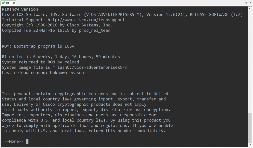
Another type of application is the interactive application. A good example is when you use telnet or SSH to access your router or switch:
These applications don’t require a lot of bandwidth but they are somewhat sensitive to delay and packet loss. Since you are typing commands and waiting for a response, a high delay can be annoying to work with. If you ever had to access a router through a satellite link, you will know what I’m talking about. Satellite links can have a one-way delay of between 500-700ms which means that when you type a few characters, there will be a short pause before you see the characters appear on your console.
With QoS, we can ensure that in case of congestion, interactive applications are served before bandwidth-hungry batch applications.
Voice and Video Application
Voice (and video) applications are the most “difficult” applications you can run on your network as it’s very sensitive to delay, jitter and packet loss. First, let me give you a quick overview of how VoIP works:
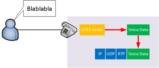
Above we have a user that is speaking. With VoIP, we use a codec that processes the analog sound into a digital signal. The analog sound is digitized for a certain time period which is usually 20 ms. With the G711 codec, each 20 ms of audio is 160 bytes of data.
The phone will then create a new IP packet with an UDP and RTP (Realtime Transport Protocol) header, adds the voice data to it and forwards the IP packet to the destination. The IP, UDP and RTP header add 40 bytes of overhead so the IP packet will be 200 bytes in total.
For one second of audio, the phone will create 50 IP packets. 50 IP packets * 200 bytes = 10000 bytes per second. That’s 80 Kbps. The G.729 codec requires less bandwidth (but with reduced audio quality) and requires only about 24 Kbps.
Bandwidth isn’t much of an issue for VoIP but delay is. If you are speaking with someone on the phone, you expect it to be real-time. If the delay is too high, the conversation becomes a bit like a walkie talkie conversation where you have to wait a few seconds before you get a reply. Jitter is an issue because the codec expects a steady stream of IP packets with voice data that it must convert back into an analog signal. Codecs can work a bit around jitter but there are limitations.
Packet loss is also an issue, too many lost packets and your conversations will have gaps in it. Voice traffic on a data network is possible but you will need QoS to ensure there is enough bandwidth and to keep the delay, jitter and packet loss under control. Here are some guidelines you can follow for voice traffic:
- One-way delay: < 150 ms.
- Jitter: <30 ms.
- Loss: < 1%
(Interactive) video traffic has similar requirements to voice traffic. Video traffic requires more bandwidth than voice traffic but this really depends on the codec and the type of video you are streaming. For example, if I record a video of my router console, 90% of the screen remains the same. The background image remains the same, only the text changes every now and then. A video with a lot of action, like a sports video, requires more bandwidth. Like voice traffic, interactive video traffic is sensitive to delay, jitter and packet loss. Here are some guidelines:
- One-way delay: 200 – 400 ms.
- Jitter: 30 – 50 ms.
- Loss: 0.1% – 1%
QoS Tools
We talked a bit about why we need QoS and different application types that have different requirements. Now let’s talk about the actual tools we can use to implement QoS:
- Classification and marking: if we want to give certain packets a different treatment, we have to identify and mark them.
- Queuing – Congestion Management: instead of having one big queue where packets are treated with FIFO, we can create multiple queues with different priorities.
- Shaping and Policing: these two tools are used to rate-limit your traffic.
- Congestion Avoidance: there are some tools we can use to manage packet loss and to reduce congestion.
Let’s walk through these tools one-by-one.
Classification and Marking
Before we can give certain packets a better treatment, we first have to identify those packets. This is called classification.

Classification can be done in a number of ways. One common way to do it is to use an access-list and match on certain values in the IP packet like the source and/or destination addresses or port numbers. For example, an access-list that matches on TCP destination port 80 is a quick way to classify all HTTP traffic.
Once the traffic is classified, it’s best practice to mark the packet.
Marking means we change one or more of the header fields in a packet or frame. For example, an IP packet has the ToS (Type of Service) field that we can use to mark the packet:
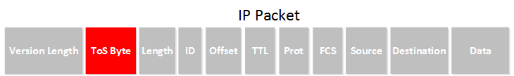
Ethernet frames don’t have such field but we do have something for trunks. The tag that is added by 802.1Q has a priority field:
Here’s an illustration to help you visualize classification and marking:

Above we see a switch with two hosts and one phone. The switch receives a number of packets from the hosts and phone and is configured to classify these packets using an access-list on its interfaces. The switch then marks the IP packets using the ToS field in the IP header.
Most IP phones mark IP packets that they create.
The reason that we use marking is that sometimes classification requires some complex access-lists / rules and can degrade performance on the router or switch that is doing classification. In the example above, the router receives marked packets so it doesn’t have to do complex classification using access-lists like the switch. It will still do classification but only has to look for marked packets.
Another useful tool for classification is NBAR (Network Based Application Recognition). NBAR is able to detect applications from your network traffic and is able to do so by looking at the content of IP packets. It allows classification that is more granular compared to what an access-list can do.
If you want to learn more about classification and marking. You can find a detailed explained of the ToS byte and IP precedence / DSCP values here. If you want to know how to configure classification, take a look at my classification on Cisco IOS router lesson and the classification/marking lesson on a catalyst switch.
Congestion Management
Every network device uses queuing. When a router receives an IP packet, it will check its routing table, decides which interface to use to send the packet and then tries to send the packet. When the interface is busy, the packet will be placed in a queue waiting for the interface to be free.
I’m talking about a router and packet but the same thing applies to switches and frames or other network devices.
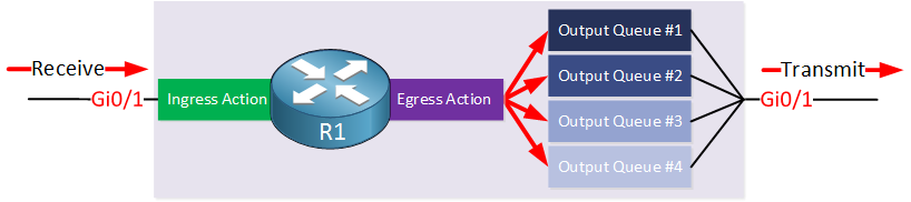
Here’s an illustration of this process:
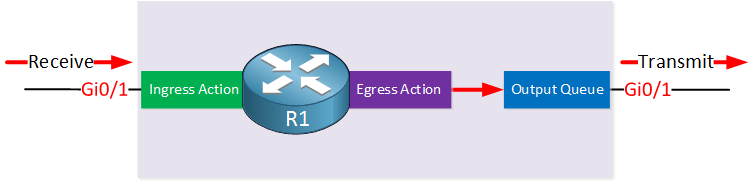
Above you can see that when the router receives a packet, it can perform one or more ingress actions, perhaps an inbound access-list that filters packets. Once the router decides where to forward the packet to, it might perform one or more egress actions. For example, NAT. The packet is then placed in an output queue, waiting for the interface to be ready and then transmitted.
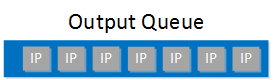
In the picture above, we only have one output queue so all packets are treated on a first come first served basis. It’s a FIFO (First In First Out) scheduler. There’s one queue and everyone must wait in line.
Most network devices offer multiple output queues. Our picture then looks like this:
The router will use classification to decide which packets go into which queue.
Round Robin Scheduling
How the queues are served, depends on the scheduler that is used. Round robin scheduling is a scheduling algorithm that cycles through the queues in order, taking turns with each queue. It might take one packet from each queue. Starting with queue 1, then queue 2, then queue 3, then queue 4 and goes back to queue 1.
Weighted round robin gives more preference to certain queues. For example, it might serve four packets from queue 1, then two packets from queue 2, then one packet from queue 3, then one packet from queue 4 and then returns to queue 1.
Cisco routers use a popular scheduler called CBWFQ (Class Based Weighted Fair Queuing) which guarantees a minimum bandwidth to each class when there is congestion. CBWFQ uses weighted round robin scheduling and allows you to configure the weighting as a percentage of the bandwidth of the interface. Here’s an illustration to help you visualize this:
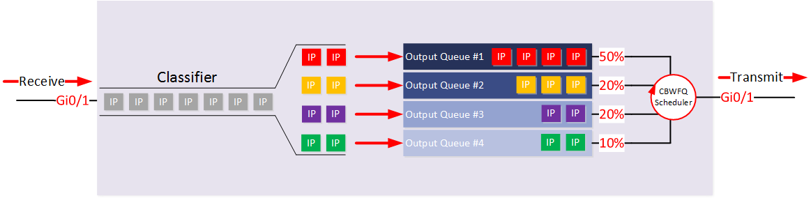
Above we see that the classifier is sending packets into the different queues. Each queue has a different percentage of the bandwidth. When there is congestion, queue 1 gets 50% of the bandwidth, queue 2 and 3 each get 20% and queue 4 gets 10%.
Low Latency Queuing
Round robin scheduling works very well for data applications as it guarantees a certain bandwidth to each queue. This doesn’t work however for delay sensitive traffic like VoIP. When the scheduler is emptying queue 2,3 and 4, all packets in queue 1 are still waiting to be served, adding delay.
In networking, this strategy doesn’t work for voice traffic that is sensitive to delay and jitter. Voice traffic has to be sent immediately and should not wait. We can solve this by adding a priority queue:
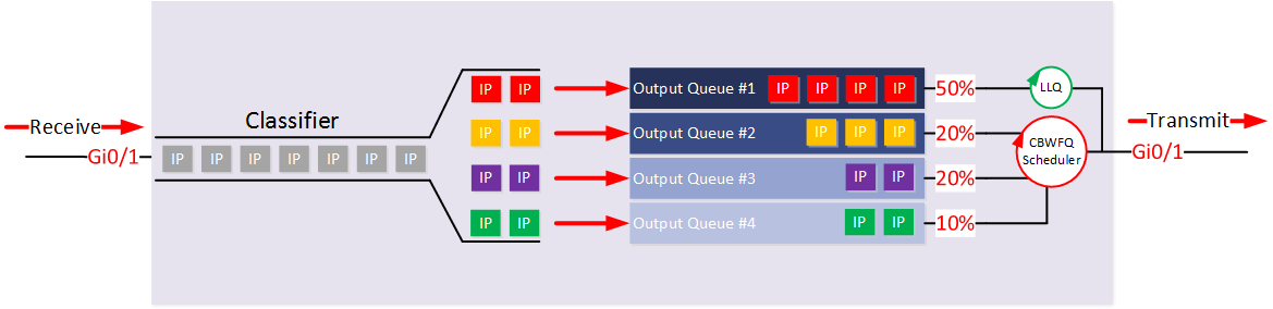
Above you can see that the first queue is now attached to LLQ. Whenever a packet is added to queue 1, it will be forwarded immediately and all other queues have to wait.
It is important to set a limit to the priority queue, otherwise, it is possible that the scheduler is so busy forwarding packets from the priority queue that the other queues are never served. When these queues get full, packets are dropped. This is called queue starvation.
Setting a limit to the priority queue does introduce another problem. What if we have so much voice traffic that we see drops in the priority queue? That would affect all voice calls. This is typically solved with CAC (Call Admission Control). In a nutshell, CAC is something you configure on your PBX which ensures that you can only have an X amount of voice calls simultaneously. If you have the capacity for 15 simultaneous voice calls, then caller 16 will get a busy signal when they try to establish a new voice call. Or the voice call gets rerouted through the PSTN.
Policing and Shaping
Shaping and policing are two QoS tools that are used to limit the bit rate. Policers do so by discarding traffic while shapers will hold packets in a queue, adding delay.
Policing
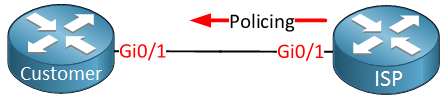
Policing is often used by ISPs who must limit the bitrate of their customers.
Let’s look at an example:
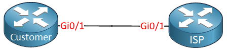
Above we have a customer and ISP router connected using Gigabit Ethernet interfaces. These interfaces run at 1000 Mbit. What if the customer only paid for a 200 Mbit connection? In this case, the ISP will drop the traffic that exceeds 200 Mbit.
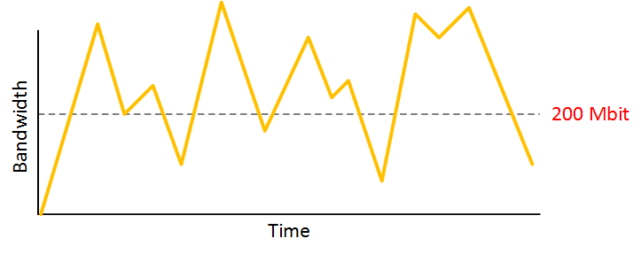
Without policing, the bit rate would look like this:
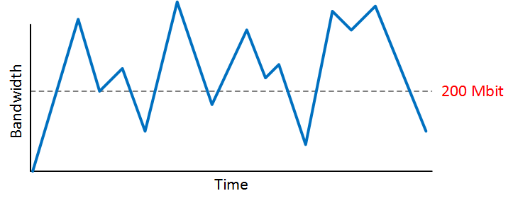
The dashed line is the bitrate the customer paid for. This is typically called the CIR (Committed Information Rate). Without policing, the customer will be able to get a higher bitrate than what they paid for. The ISP will configure inbound policing:
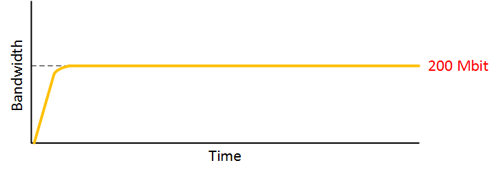
With policing enabled, the bitrate looks like this:
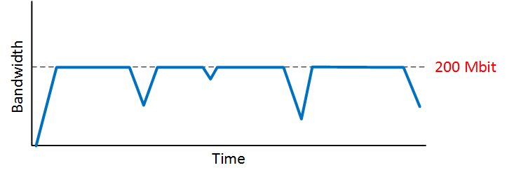
200 Mbit is now a hard limit which might not be completely fair to the customer. During a longer period of time, it’s impossible to get an average bit rate of 200 Mbit. Because of this, policing is often implemented so you are allowed to “burst” your traffic for a short while after inactivity:
Above you can see that after a longer time of inactivity, we are allowed to exceed our CIR rate of 200 Mbit for a short while before the policer kicks in.
Instead of dropping packets right away, policers can also be configured to re-mark your packets to a lower priority. Your traffic won’t be dropped right away, but maybe somewhere further down the network.
If you want a detailed explanation of how policing works, you can take a look at my introduction to policing lesson.
Shaping
In the previous example, you have seen how an ISP might use policing to drop your traffic. If the customer has a CIR rate of 200 Mbit and they exceed this rate, their traffic gets dropped.
To prevent this from happening, we can implement shaping on the customer side. The shaper will queue messages, delaying them to a certain CIR rate.
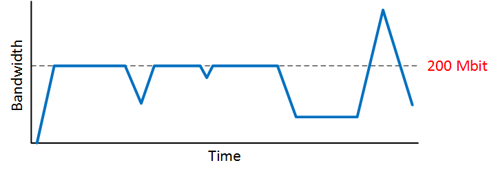
Without shaping, the bit rate that the customer sends might look like this:
Everything above the dashed line will then be dropped by the ISP’s policer. Once we configure the shaper, our bit rate will look like this:
Everything is queued and delayed so we don’t exceed the 200 Mbit bitrate. This prevents our traffic from getting dropped at the ISP.
The shaper solves one issue but it might introduce another issue. Let me give you an example of how a shaper works:
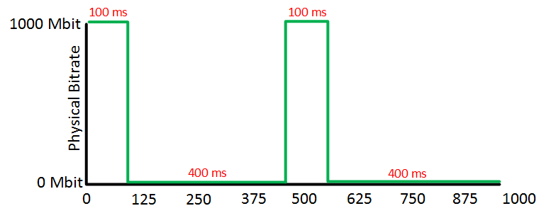
We have our CIR rate of 200 Mbit, the physical interface has a bit rate of 1000 Mbit. The interface is only capable of sending traffic at 1000 Mbit. In one second, the shaper will send 20% of the timer and wait 80% of the time. This way, we will achieve our target rate of 200 Mbit.
1000 Mbit is 1000 million bits that are sent in 1000 ms (one second). If we want to hit our target rate of 200 Mbit, we should only send 200 million bits in one second. In the picture above you can see the shaper sends traffic for a duration of 100 ms, then waits 400 ms, sends traffic for 100 ms, then waits 400 ms and the cycle is complete for one second.
During that 400 ms pause, packets are queued. When we talked about VoIP, I explained that the maximum one-way delay for voice packets should be below 150 ms so this is going to be a problem. Luckily, the time interval (called the Tc) of a shaper can be configured. For example, we could also send for 10 ms and then wait for 40 ms:
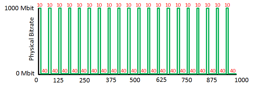
Above you can see we have 20 moments where we send for 10 ms. 20 x 10 = 200 ms in total. We have 20 pauses of 40 ms, 20x 40 = 800 ms in total. Voice packets will only have to wait for a maximum of 40 ms this way.
A recommendation for voice traffic is to use a maximum pause of 10 ms. This way, voice traffic is only delayed for 10 ms because of the shaper.
For a detailed explanation of how a shaper works, you can check my traffic shaping explained lesson.
Congestion Avoidance
To understand congestion avoidance, we first have to talk about TCP and its window size.
TCP uses flow control using a window size where the receiver tells the sender how many bytes to send before expecting an acknowledgment. The higher the window size, the less overhead and the higher the throughput will be.
Here’s how the TCP slow-start mechanism works:
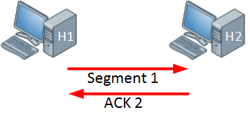
TCP can use a Congestion Window (CWND) and receiver window (RWND) to control the transfer rate and avoid network congestion. When there is no packet loss, the window size will increase, doubling every time. Below you can see that hat H2 receives a single TCP segment which is acknowledged.
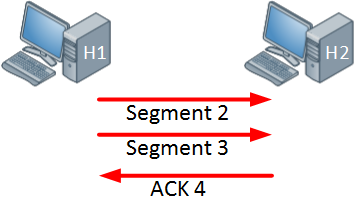
H1 increases the window size and now we send two TCP segments before the ACK is returned:
The window size doubles again, and we send four TCP segments before the ACK is returned:
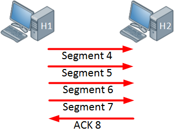
We keep doubling the window size until TCP segments get lost or when we hit the receiver’s advertised window size (RWND). For each TCP segment that is lost, the TCP window size is shrunk by half. If multiple TCP segments are lost, each time the window size is shrunk by half.
If you want to learn more about the TCP window size and what it looks like in action, take a look at our TCP window size scaling lesson.
Now let’s take a closer look at queuing and I’ll explain how the TCP window size applies to queuing. Here’s an example of an output queue:
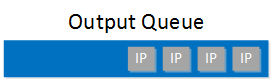
The output queue above has four packets, there is still room for more packets. The interface is quite busy so a bit later, more packets are queued:
Right now the queue is full so if another packet arrives, it will be dropped:
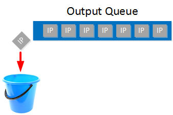
This is called tail drop. To deal with this, we can use a congestion avoidance tool like WRED. These tools will monitor the output queue and once it’s at a certain level, it will drop TCP segments, hoping that by reducing the window size, TCP connections will slow down so that we can reduce congestion and prevent tail drop.
Here’s an illustration:
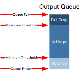
When the queue is empty, we don’t drop any packets. Once the queue fills and it’s between the minimum and maximum threshold, we drop a small percentage of our packets. Once we exceed the maximum threshold, we drop all packets.
The congestion avoidance tool can randomly drop packets, or we can configure it to give certain packets a different treatment based on their marking.
Conclusion
In this lesson, you have learned the basics of QoS (Quality of Service):
- Why we need QoS.
- The characteristics of network traffic:
- bandwidth
- delay
- jitter
- loss
- The different application types we have and how they are affected by bandwidth, delay, jitter and loss.
- The QoS tools we have:
- classification and marking
- queuing / congestion management
- shaping and policing
- congestion avoidance
- How classification is used to identify network traffic and why we mark traffic.
- Why network devices have one or more output queues.
- The different scheduling algorithms and why we need a priority queue for real-time traffic like VoIP.
- How shaping and policing limit the bitrate.
- How congestion avoidance tools drop packets in the output queue, hoping to reduce the TCP window size and prevent congestion.
I hope you enjoyed this lesson, if you have any questions feel free to leave a comment below.